Sql Training - 10

 Introduction to SQL INTERSECT operator

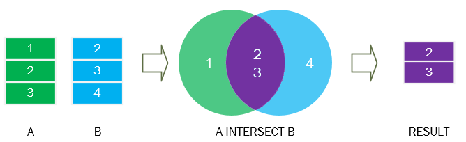
The INTERSECT operator is a set operator that returns distinct rows of two or more result sets from SELECT statements.

Suppose, we have two tables: A(1,2) and B(2,3).

The following picture illustrates the intersection of A & B tables.

The purple section is the intersection of the green and blue result sets.

Like the UNION operator, the INTERSECT operator removes the duplicate rows from the final result set.

To use the INTERSECT operator, the columns of the SELECT statements must follow the rules:

• The data types of columns must be compatible.
• The number of columns and their orders in the SELECT statements must be the same.

SQL INTERSECT with ORDER BY example

To sort the result set returned by the INTERSECT operator, you place the ORDER BY clause at the end of all statements.

For example, the following statement applies the INTERSECT operator to the A and B tables and sorts the combined result set by the id column in descending order.

SELECT
	id
FROM
	a 
INTERSECT
SELECT
	id
FROM
	b
ORDER BY id DESC;
Code language: SQL (Structured Query Language) (sql)

Introduction to SQL MINUS operator

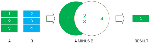
Besides the UNION, UNION ALL, and INTERSECT operators, SQL provides us with the MINUS operator that allows you to subtract one result set from another result set.

To use the MINUS operator, you write individual SELECT statements and place the MINUS operator between them. The MINUS operator returns the unique rows produced by the first query but not by the second one.

The following picture illustrates the MINUS operator.

To make the result set, the database system performs two queries and subtracts the result set of the first query from the second one.

In order to use the MINUS operator, the columns in the SELECT clauses must match in number and must have the same or, at least, convertible data type.

We often use the MINUS operator in ETL. An ETL is a software component in data warehouse system. ETL stands for Extract, Transform, and Load. ETL is responsible for loading data from the source systems into the data warehouse system.

After complete loading data, we can use the MINUS operator to make sure that the data has been loaded fully by subtracting data in target system from the data in the source system.

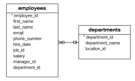
Each employee has zero or more dependents while each dependent depends on one and only one employees. The relationship between the dependents and employees is the one-to-many relationship.

The employee_id column in the dependents table references to the employee_id column in the  employees table.

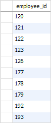
You can use the MINUS operator to find the employees who do not have any dependents. To do this, you subtract the employee_id result set in the  employees table from the employee_id result set in the dependents table.

The following query illustrates the idea:

SELECT 
    employee_id
FROM
    employees 
MINUS 
SELECT 
    employee_id
FROM
    dependents;


SQL  MINUS with ORDER BY example
To sort the result set returned by the MINUS operator, you place the ORDER BY clause at the end of the last SELECT statement.
For example, to sort the employees who do not have any dependents, you use the following query:
SELECT 
    employee_id
FROM
    employees 
MINUS 
SELECT 
    employee_id
FROM
    dependents
ORDER BY employee_id;
Code language: SQL (Structured Query Language) (sql)

Data Manipulation Statements 

Save and discard changes with the COMMIT and ROLLBACK statements Explain read consistency 

Other Schema Objects 

Create a simple and complex view 

Retrieve data from views 

Introduction to the SQL Views

A relational database consists of multiple related tables e.g., employees, departments, jobs, etc. When you want to see the data of these tables, you use the SELECT statement with JOIN or UNION clauses.

SQL provides you with another way to see the data is by using the views.  A view is like a virtual table produced by executing a query. The relational database management system (RDBMS) stores a view as a named SELECT in the database catalog.

Whenever you issue a SELECT statement that contains a view name, the RDBMS executes the view-defining query to create the virtual table. That virtual table then is used as the source table of the query.

Why do you need to use the views

Views allow you to store complex queries in the database. For example, instead of issuing a complex SQL query each time you want to see the data, you just need to issue a simple query as follows:

SELECT column_list
FROM view_name;
Code language: SQL (Structured Query Language) (sql)

Views help you pack the data for a specific group of users. For example, you can create a view of salary data for the employees for Finance department.

Views help maintain database security. Rather than give the users access to database tables, you create a view to revealing only necessary data and grant the users to access to the view.

Creating SQL views

To create a view, you use the CREATE VIEW statement as follows:

CREATE VIEW view_name 
AS
SELECT-statement
Code language: SQL (Structured Query Language) (sql)

First, specify the name of the view after the CREATE VIEW clause.

Second, construct a SELECT statement to query data from multiple tables.

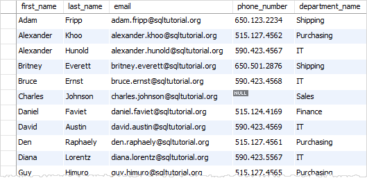
For example, the following statement creates the employee contacts view based on the data of the employees and departments tables.

CREATE VIEW employee_contacts AS
    SELECT 
        first_name, last_name, email, phone_number, department_name
    FROM
        employees e
            INNER JOIN
        departments d ON d.department_id = e.department_id
    ORDER BY first_name;
Code language: SQL (Structured Query Language) (sql)

By default, the names of columns of the view are the same as column specified in the SELECT statement. If you want to rename the columns in the view, you include the new column names after the CREATE VIEW clause as follows:

CREATE VIEW view_name(new_column_list) 
AS
SELECT-statement;
Code language: SQL (Structured Query Language) (sql)

For example, the following statement creates a view whose column names are not the same as the column names of the base tables.

CREATE VIEW payroll (first_name , last_name , job, compensation) AS
    SELECT 
        first_name, last_name, job_title, salary
    FROM
        employees e
            INNER JOIN
        jobs j ON j.job_id= e.job_id
    ORDER BY first_name;
Code language: SQL (Structured Query Language) (sql)

Querying data from views

Querying data from views is the same as querying data from tables. The following statement selects data from the employee_contacts view.

SELECT 
    *
FROM
    employee_contacts;
Code language: SQL (Structured Query Language) (sql)

Of course, you can apply filtering or grouping as follows:

SELECT 
    job, 
    MIN(compensation), 
    MAX(compensation), 
    AVG(compensation)
FROM
    payroll
WHERE
    job LIKE 'A%'
GROUP BY job;
Code language: SQL (Structured Query Language) (sql)

Modifying SQL views

To modify a view, either adding new columns to the view or removing columns from a view, you use the same CREATE OR REPLACE VIEW statement.

CREATE OR REPLACE view_name AS
SELECT-statement;
Code language: SQL (Structured Query Language) (sql)

The statement creates a view if it does not exist or change the current view if the view already exists.

For example, the following statement changes the payroll view by adding the department column and rename the compensation column to salary column.

CREATE OR REPLACE VIEW payroll (first_name , last_name , job , department , salary) AS
    SELECT 
        first_name, last_name, job_title, department_name, salary
    FROM
        employees e
            INNER JOIN
        jobs j ON j.job_id = e.job_id
            INNER JOIN
        departments d ON d.department_id = e.department_id
    ORDER BY first_name;
Code language: SQL (Structured Query Language) (sql)

SELECT 
    *
FROM
    payroll;
Code language: SQL (Structured Query Language) (sql)

Removing SQL views

To remove a view from the database, you use the DROP VIEW statement:

DROP VIEW view_name;
Code language: SQL (Structured Query Language) (sql)

The DROP VIEW statement deletes the view only, not the base tables.

For example, to remove the payroll view, you use the following statement:

DROP VIEW payroll;

Create and maintain indexes 

Why SQL Index?

The following reasons tell why Index is necessary in SQL:

• SQL Indexes can search the information of the large database quickly.
• This concept is a quick process for those columns, including different values.
• This data structure sorts the data values of columns (fields) either in ascending or descending order. And then, it assigns the entry for each value.
• Each Index table contains only two columns. The first column is row_id, and the other is indexed-column.
• When indexes are used with smaller tables, the performance of the index may not be recognized.

Create an INDEX

In SQL, we can easily create the Index using the following CREATE Statement:

1. CREATE INDEX Index_Name ON Table_Name ( Column_Name);  

Here, Index_Name is the name of that index that we want to create, and Table_Name is the name of the table on which the index is to be created. The Column_Name represents the name of the column on which index is to be applied.

1. CREATE INDEX index_state ON Employee (Emp_State);  

Suppose we want to create an index on the combination of the Emp_city and the Emp_State column of the above Employee table. For this, we have to use the following query:

1. CREATE INDEX index_city_State ON Employee (Emp_City, Emp_State);  

Create UNIQUE INDEX

Unique Index is the same as the Primary key in SQL. The unique index does not allow selecting those columns which contain duplicate values.

This index is the best way to maintain the data integrity of the SQL tables.

Syntax for creating the Unique Index is as follows:

1. CREATE UNIQUE INDEX Index_Name ON Table_Name ( Column_Name);  

Introduction to SQL Server clustered indexes

The following statement creates a new table named production.parts that consists of two columns part_id and part_name:

CREATE TABLE production.parts(
    part_id   INT NOT NULL, 
    part_name VARCHAR(100)
);
Code language: CSS (css)

And this statement inserts some rows into the production.parts table:

INSERT INTO 
    production.parts(part_id, part_name)
VALUES
    (1,'Frame'),
    (2,'Head Tube'),
    (3,'Handlebar Grip'),
    (4,'Shock Absorber'),
    (5,'Fork');
Code language: JavaScript (javascript)

The production.parts table does not have a primary key. Therefore SQL Server stores its rows in an unordered structure called a heap.

When you query data from the production.parts table, the query optimizer needs to scan the whole table to search.

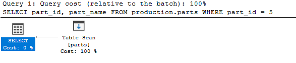
For example, the following SELECT statement finds the part with id 5:

SELECT 
    part_id, 
    part_name
FROM 
    production.parts
WHERE 
    part_id = 5;

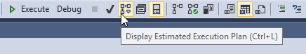
If you display the estimated execution plan in SQL Server Management Studio, you’ll see how SQL Server come up with the following query plan:

Note that to display the estimated execution plan in SQL Server Management Studio, you click the Display Estimated Execution Plan button or select the query and press the keyboard shortcut Ctrl+L:

Because the production.parts table has only five rows, the query executes very fast. However, if the table contains a large number of rows, it’ll take a lot of time and resources to search for data.

To resolve this issue, SQL Server provides a dedicated structure to speed up the retrieval of rows from a table called index.

SQL Server has two types of indexes: clustered index and non-clustered index. We will focus on the clustered index in this tutorial.

A clustered index stores data rows in a sorted structure based on its key values. Each table has only one clustered index because data rows can be only sorted in one order. A table that has a clustered index is called a clustered table.

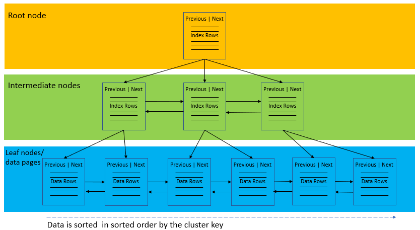
The following picture illustrates the structure of a clustered index:

A clustered index organizes data using a special structured so-called B-tree (or balanced tree) which enables searches, inserts, updates and deletes in logarithmic amortized time.

In this structure, the top node of the B-tree is called the root node. The nodes at the bottom level are called the leaf nodes. Any index levels between the root and the leaf nodes are known as intermediate levels.

In the B-Tree, the root node and intermediate level nodes contain index pages that hold index rows. The leaf nodes contain the data pages of the underlying table. The pages in each level of the index are linked using another structure called a doubly-linked list.

SQL Server Clustered Index and Primary key constraint

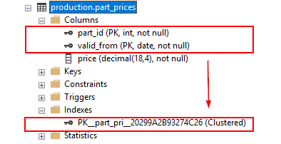
When you create a table with a primary key, SQL Server automatically creates a corresponding clustered index that includes primary key columns.

This statement creates a new table named production.part_prices with a primary key that includes two columns: part_id and valid_from.

CREATE TABLE production.part_prices(
    part_id int,
    valid_from date,
    price decimal(18,4) not null,
    PRIMARY KEY(part_id, valid_from) 
);
Code language: JavaScript (javascript)

If you add a primary key constraint to an existing table that already has a clustered index, SQL Server will enforce the primary key using a non-clustered index:

This statement defines a primary key for the production.parts table:

ALTER TABLE production.parts
ADD PRIMARY KEY(part_id);
Code language: CSS (css)

SQL Server created a non-clustered index for the primary key.

Using SQL Server CREATE CLUSTERED INDEX statement to create a clustered index.

When a table does not have a primary key, which is very rare, you can use the CREATE CLUSTERED INDEX statement to add a clustered index to it.

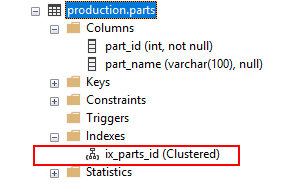
The following statement creates a clustered index for the production.parts table:

CREATE CLUSTERED INDEX ix_parts_id
ON production.parts (part_id);  
Code language: CSS (css)

If you open the Indexes node under the table name, you will see the new index name ix_parts_id with type Clustered.

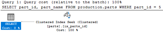
When executing the following statement, SQL Server traverses the index (Clustered Index Seek) to locate the rows, which is faster than scanning the whole table.

SELECT 
    part_id, 
    part_name
FROM 
    production.parts
WHERE 
    part_id = 5;

Table Variable

 

A Table Variable is a variable that can store the complete table of the data inside it. It is similar to a Table Variable but as I said a Table Variable is a variable. So how do we declare a variable in SQL? Using the @ symbol. The same is true for a Table Variable. so the syntax of the Table Variable is as follows:

Declare @TempTable TABLE(      

id int,    

Name varchar(20)      

)      

  

insert into @TempTable values(1,'Sourabh Somani')  

insert into @TempTable values(2,'Shaili Dashora')  

insert into @TempTable values(3,'Divya Sharma')  

insert into @TempTable values(4,'Swati Soni')  

  

Select * from @TempTable  

 

Difference between temporary tables and Table Variable

 

There are a difference between temporary tables and temporary variables, it is:

1. A Table Variable is not available after execution of the complete query so you cannot run a single query but a temporary table is available after executing the query.
   
   For example:
   
   
   
   
2. A Transaction (Commit and Rollback) operation is not possible in a Table Variable but in a temporary table we can perform transactiona (Commit and Rollback).
   
   For example:
   
   1. Declare @TempTable TABLE(      
   2. id int,    
   3. Name varchar(20)      
   4. )      
   5. begin tran T  
   6. insert into @TempTable values(1,'Sourabh Somani')  
   7. insert into @TempTable values(2,'Shaili Dashora')  
   8. insert into @TempTable values(3,'Divya Sharma')  
   9. insert into @TempTable values(4,'Swati Soni')  
   10. commit tran T  
   11. Select * from @TempTable  
   
   
   or 
   
   1. Declare @TempTable TABLE(      
   2. id int,    
   3. Name varchar(20)      
   4. )      
   5. begin tran T  
   6. insert into @TempTable values(1,'Sourabh Somani')  
   7. insert into @TempTable values(2,'Shaili Dashora')  
   8. insert into @TempTable values(3,'Divya Sharma')  
   9. insert into @TempTable values(4,'Swati Soni')  
   10. rollback tran T  
   11. Select * from @TempTable  
   
   

Important Points about Table Variables

• The same as a temporary table.
• Single query cannot be executed.
• When we want to perform a few operations then use a Table Variable otherwise if it is a huge amount of data operation then use a temporary table.
• Commit and Rollback (Transaction) cannot be possible with Table Variables so if you want to perform a transaction operation then always go with temporary tables.

What are scalar functions

SQL Server scalar function takes one or more parameters and returns a single value.

The scalar functions help you simplify your code. For example, you may have a complex calculation that appears in many queries. Instead of including the formula in every query, you can create a scalar function that encapsulates the formula and uses it in each query.

Creating a scalar function

To create a scalar function, you use the CREATE FUNCTION statement as follows:

CREATE FUNCTION [schema_name.]function_name (parameter_list)
RETURNS data_type AS
BEGIN
    statements
    RETURN value
END
Code language: SQL (Structured Query Language) (sql)

In this syntax:

• First, specify the name of the function after the CREATE FUNCTION keywords. The schema name is optional. If you don’t explicitly specify it, SQL Server uses dbo by default.
• Second, specify a list of parameters surrounded by parentheses after the function name.
• Third, specify the data type of the return value in the RETURNS statement.
• Finally, include a RETURN statement to return a value inside the body of the function.

The following example creates a function that calculates the net sales based on the quantity, list price, and discount:

CREATE FUNCTION sales.udfNetSale(
    @quantity INT,
    @list_price DEC(10,2),
    @discount DEC(4,2)
)
RETURNS DEC(10,2)
AS 
BEGIN
    RETURN @quantity * @list_price * (1 - @discount);
END;
Code language: SQL (Structured Query Language) (sql)

Later on, we can use this to calculate net sales of any sales order in the order_items from the sample database.

After creating the scalar function, you can find it under Programmability > Functions > Scalar-valued Functions as shown in the following picture:

Calling a scalar function

You call a scalar function like a built-in function. For example, the following statement demonstrates how to call the udfNetSale function:

SELECT 
    sales.udfNetSale(10,100,0.1) net_sale;
Code language: SQL (Structured Query Language) (sql)

Here is the output:

The following example illustrates how to use the sales.udfNetSale function to get the net sales of the sales orders in the order_items table:

SELECT 
    order_id, 
    SUM(sales.udfNetSale(quantity, list_price, discount)) net_amount
FROM 
    sales.order_items
GROUP BY 
    order_id
ORDER BY
    net_amount DESC;
Code language: SQL (Structured Query Language) (sql)

The following picture shows the partial output:

Modifying a scalar function

To modify a scalar function, you use the ALTER instead of the CREATE keyword. The rest statements remain the same:

ALTER FUNCTION [schema_name.]function_name (parameter_list)
    RETURN data_type AS
    BEGIN
        statements
        RETURN value
    END
Code language: SQL (Structured Query Language) (sql)

Note that you can use the CREATE OR ALTER statement to create a user-defined function if it does not exist or to modify an existing scalar function:

CREATE OR ALTER FUNCTION [schema_name.]function_name (parameter_list)
        RETURN data_type AS
        BEGIN
            statements
            RETURN value
        END
Code language: SQL (Structured Query Language) (sql)

Removing a scalar function

To remove an existing scalar function, you use the DROP FUNCTION statement:

DROP FUNCTION [schema_name.]function_name;
Code language: SQL (Structured Query Language) (sql)

For example, to remove the sales.udfNetSale function, you use the following statement:

DROP FUNCTION sales.udfNetSale;
Code language: SQL (Structured Query Language) (sql)

SQL Server scalar function notes

The following are some key takeaway of the scalar functions:

• Scalar functions can be used almost anywhere in T-SQL statements.
• Scalar functions accept one or more parameters but return only one value, therefore, they must include a RETURN statement.
• Scalar functions can use logic such as IF blocks or WHILE loops.
• Scalar functions cannot update data. They can access data but this is not a good practice.
• Scalar functions can call other functions

What is a table-valued function in SQL Server

A table-valued function is a user-defined function that returns data of a table type. The return type of a table-valued function is a table, therefore, you can use the table-valued function just like you would use a table.

Creating a table-valued function

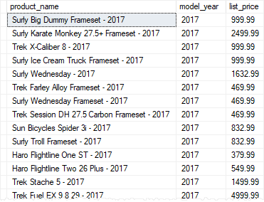
The following statement example creates a table-valued function that returns a list of products including product name, model year and the list price for a specific model year:

CREATE FUNCTION udfProductInYear (
    @model_year INT
)
RETURNS TABLE
AS
RETURN
    SELECT 
        product_name,
        model_year,
        list_price
    FROM
        production.products
    WHERE
        model_year = @model_year;
Code language: SQL (Structured Query Language) (sql)

The syntax is similar to the one that creates a user-defined function.

The RETURNS TABLE specifies that the function will return a table. As you can see, there is no BEGIN...END statement. The statement simply queries data from the production.products table.

The udfProductInYear function accepts one parameter named @model_year of type INT. It returns the products whose model years equal @model_year parameter.

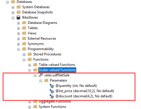
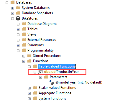
Once the table-valued function is created, you can find it under Programmability > Functions > Table-valued Functions as shown in the following picture:

The function above returns the result set of a single SELECT statement, therefore, it is also known as an inline table-valued function.

Executing a table-valued function

To execute a table-valued function, you use it in the FROM clause of the SELECT statement:

SELECT 
    * 
FROM 
    udfProductInYear(2017);
Code language: SQL (Structured Query Language) (sql)

In this example, we selected the products whose model year is 2017.

You can also specify which columns to be returned from the table-valued function as follows:

SELECT 
    product_name,
    list_price
FROM 
    udfProductInYear(2018);
Code language: SQL (Structured Query Language) (sql)

Here is the partial output:

Modifying a table-valued function

To modify a table-valued function, you use the ALTER instead of CREATE keyword. The rest of the script is the same.

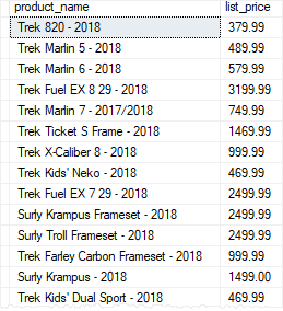
For example, the following statement modifies the udfProductInYear by changing the existing parameter and adding one more parameter:

ALTER FUNCTION udfProductInYear (
    @start_year INT,
    @end_year INT
)
RETURNS TABLE
AS
RETURN
    SELECT 
        product_name,
        model_year,
        list_price
    FROM
        production.products
    WHERE
        model_year BETWEEN @start_year AND @end_year
Code language: SQL (Structured Query Language) (sql)

The udfProductInYear function now returns products whose model year between a starting year and an ending year.

The following statement calls the udfProductInYear function to get the products whose model years are between 2017 and 2018:

SELECT 
    product_name,
    model_year,
    list_price
FROM 
    udfProductInYear(2017,2018)
ORDER BY
    product_name;
Code language: SQL (Structured Query Language) (sql)

Here is the partial output:

Management of Schema Objects 

Add, Modify and Drop a Column

Add, Drop and Defer a Constraint 

How to enable and Disable a Constraint? 

Create and Remove Indexes 

Create a Function-Based Index 

Perform Flashback Operations 

Create an External Table by Using ORACLE_LOADER and by Using ORACLE_DATAPUMP Query External Tables 

Manage Objects with Data Dictionary Views 

Explain the data dictionary 

Use the Dictionary Views 

USER_OBJECTS and ALL_OBJECTS Views 

Table and Column Information 

Query the dictionary views for constraint information 

Query the dictionary views for view, sequence, index, and synonym information Add a comment to a table 

Query the dictionary views for comment information 

Manipulate Large Data Sets

Use Subqueries to Manipulate Data 

Retrieve Data Using a Subquery as Source 

Insert Using a Subquery as a Target 

Usage of the WITH CHECK OPTION Keyword on DML Statements List the types of Multitable INSERT Statements 

Use Multitable INSERT Statements 

Merge rows in a table 

Track Changes in Data over a period of time 

---------

Create, maintain, and use sequences 

Create private and public synonyms 

Control User Access 

Differentiate system privileges from object privileges Create Users 

Grant System Privileges 

Create and Grant Privileges to a Role 

Change Your Password 

Grant Object Privileges 

How to pass on privileges? 

Revoke Object Privileges 

------------

Data Management in Different Time Zones 

Time Zones 

CURRENT_DATE, CURRENT_TIMESTAMP, and LOCALTIMESTAMP þÿCompare Date and Time in a Session  s Time Zone DBTIMEZONE and SESSIONTIMEZONE 

Difference between DATE and TIMESTAMP 

INTERVAL Data Types 

Use EXTRACT, TZ_OFFSET, and FROM_TZ 

Invoke TO_TIMESTAMP,TO_YMINTERVAL and TO_DSINTERVAL

Retrieve Data Using Sub-queries 

Multiple-Column Subqueries 

Pairwise and Nonpairwise Comparison 

Scalar Subquery Expressions 

Solve problems with Correlated Subqueries 

Update and Delete Rows Using Correlated Subqueries The EXISTS and NOT EXISTS operators 

Invoke the WITH clause 

The Recursive WITH clause 

Regular Expression Support 

Use the Regular Expressions Functions and Conditions in SQL Use Meta Characters with Regular Expressions 

Perform a Basic Search using the REGEXP_LIKE function Find patterns using the REGEXP_INSTR function Extract Substrings using the REGEXP_SUBSTR function Replace Patterns Using the REGEXP_REPLACE function Usage of Sub-Expressions with Regular Expression Support

Implement the REGEXP_COUNT function